While it may be true that Evolutionary Anthropologists consider themselves scientists…

Casey Roulette, a former PhD student of mine who is now an assistant professor at San Diego State University, recently received an email from a member of the Biology Department who was irate that Casey’s evolutionary anthropology course, Evolution of Human Nature, was being considered to fulfill “Natural Sciences” GE reqs. She informed him that she had complained to her Chair, who in turn complained to the Dean of the College of Sciences, and that “Both will be preparing a letter to be sent to the GE committee indicating that the College of Sciences does not support this course as a GE course.” The email concluded:

While it may be true that Evolutionary Anthropologists consider themselves scientists and use the terms evolution and evolutionary, the “Evolutionary Biology” represented in this course does not reflect or represent modern Evolutionary Biology as defined by Evolutionary Biologists.

In our meeting with the Instructor, who I know is an Assistant Professor, I thought it was not collegial to point out that his views on “evolutionary anthropology” are not considered accurate by those of us trained in Evolutionary Biology.

…

It is deeply concerning that students could leave this campus with such an erroneous understanding of such a fundamental scientific process.

She attached an evaluation from the SDSU Department of Biology. The first part argued that, on programmatic grounds, the course did a good job fulfilling the Social Science reqs. I agree.

The second part, however, echoed the email, arguing on scientific grounds that the course did not qualify as a GE course in the Natural Sciences because it presented a view of biology that was incomplete, biased and incorrect.

That’s odd. If true, Casey’s course shouldn’t qualify for GE in either the Social or Natural Sciences. In fact, his course shouldn’t be taught at all.

SDSU biologists’ first concern was that Casey presents evolution as synonymous with adaptation:

The “Evolutionary” approach presented in this class seems to present biological evolution as synonymous with adaptation via natural selection. Natural selection is but one of the five evolutionary forces that determine patterns of variation within and among species. For example, no information is provided on the very important role of Random Genetic Drift in shaping genetic variation.

The practice of interpreting biological patterns only through the lens of adaptation has been labeled the “Adaptionist program”. For four decades, biologists have recognized the folly of this approach. The phrase “The Fallacy of Intuitive Evolutionary Thinking” has also been used to describe the assumption that every biological feature has been optimized by selection. Evolutionary biologists accept the power of Darwinian natural selection but we do so understanding that natural selection is a complex process.

Their second concern was that Casey does not discuss genetic drift, and its role in human evolution:

There is no discussion of the Neutral and Nearly Neutral models of Evolution, which have been the dominant models of molecular evolution for 50 years.

It is also well established that Homo sapiens has an effective population size (Ne) of approximately 10,000. With such a small effective population size it is widely understood (among evolutionary biologists) that selection is inefficient in H. sapiens. Because of this evolutionary biologists would expect to see high levels of both fixed and segregating neutral and nearly neutral (slightly deleterious) alleles within and between human populations. Our most current understanding of genetic variation in does not fit in to the pan selectionist approach presented in this class.

By “the pan selectionist approach” I suppose they are referring to the focus of Casey’s course, Human Behavioral Ecology (HBE).

The debate over adaptationism, however, is an ongoing debate, one that began more than a century ago. Each side has involved towering figures in evolutionary biology like Fisher, Wright, Williams, Hamilton, Maynard Smith, Gould, Lewontin, and Kimura.

The neutralist–selectionist debate — are patterns of genetic variation primarily explained by random genetic drift or natural selection? — is, again, a debate.

Does Casey’s syllabus present both sides of these debates?

The assigned reading in Week 2 of the course is Stephen Jay Gould’s Sociobiology: the art of storytelling. It was Gould, of course, who with co-author Richard Lewontin, introduced the phrase “Adaptationist Programme” in their hugely influential article The spandrels of San Marco and the Panglossian paradigm: a critique of the adaptationist programme. One of Gould’s key points is the important role of genetic drift.

More importantly, one of two required books for the course is Laland and Brown’s Sense and nonsense: Evolutionary perspectives on human behaviour. I would count Laland as a consistent critic of the adaptationist program (in favor of his alternative, niche construction, developed in collaboration with eminent population geneticist Marcus Feldman) whose book is a good-faith effort to describe the controversies as they apply to human evolution. Laland and Brown do discuss neutral theory, drift and molecular evolution, especially their intriguing parallels with cultural evolution. Casey also assigned chapter 7 of Evolution of Human Behavior, by Agustin Fuentes, who I would also count as a critic of adaptationism.

Although Casey’s course focuses on the evolution of the human behavioral phenotype and not molecular evolution, I see no evidence that the course, which also assigns Wrangham’s Demonic males, is giving students a biased overview of the debates over adaptationism and neutralism vs. selectionism.

And it’s not quite true that neutral models “have been the dominant models of molecular evolution for 50 years.” Instead, the intense debate has perhaps resulted in a consensus. According to evolutionary geneticists Charlesworth and Charlesworth, “From the late 1980s, the neutral theory came increasingly to be used as a null hypothesis, against which alternative hypotheses could be tested, including the models of the effects of selection on neutral or nearly neutral variability at linked sites….”, a point also made by Masatoshi Nei and Kimura himself.

At this point I should admit that I’m an unreconstructed ultra-Darwinian Fundamentalist who, each night, reads his daughters passages from the Selfish Gene. Depression is an adaptation! Drug use is an adaptation! This was my logo for the first iteration of this blog:

Pangloss

Casey, what’s with the balanced overview? Did I teach you nothing?

In my view, critics of adaptationism have things backwards. For adaptationists, the question is not, do constraints and noise play an important role in organism structure? The question is, why don’t constraints and noise dominate organism structure? Constraints and noise permeate physical processes, yet organisms — intricate machines that surpass all human technology — somehow manage to make precise copies of themselves in hostile environments. It is exactly this problem, as I discuss in a bit more detail here, that adaptationists are trying to solve.

The population genetics folks have it right: random genetic variation, and more generally, noise, by-products, constraints, and thermodynamically favored physics and chemistry, should always be the null hypotheses that an adaptationist hypothesis needs to beat.

Course approval at SDSU is a pretty trivial topic, but the evidence for noise vs. selection in the human genome is not. I therefore thought I would use this post as an opportunity to learn a bit more about it. It’s not meant to be a comprehensive review, just a taste of some major issues. I’m not a genetics guy — far from it — so if I make any mistakes, let me know in the comments.

Population genetics 101

The SDSU biologists’ argument that, due to a small effective population size (\(N_e\)), selection is “inefficient” in H. sapiens rests on a classic result from population genetics. Each generation is a sample of alleles from the previous generation. A particular allele might decrease the probability that individuals with the allele reproduce (negative selection), increase the probability (positive selection), or have no effect (neutral). This effect is quantified by the selection coefficient, \(s\), which is the difference in fitness, \(W\), between two alleles, the wild type, A, and a mutant type, B:

\[ s = W_B - W_A \]

Even when \(s=0\), the frequencies of A and B will change at least a little bit from generation to generation due to random differences in the survival and reproduction of individuals with A vs. B. On average, however, the frequency of a neutral mutant allele in a new generation is, under some strong simplifying assumptions, simply the frequency of the allele in the original generation.

If the population is small, however, then the “sample size” is small. Just as we learn in statistics, the smaller the sample size, the larger the variance in the “sample estimate.” Thus, in small populations, the frequency of a neutral allele will bounce around from generation to generation more than it would in large populations, eventually going to either 0 (lost) or 1 (fixed). In particular, the frequency of a new mutation is small, so there’s a good chance that it won’t be “sampled,” and will thus be lost.

But what if the allele isn’t neutral? Naively, if an allele has a negative effect on fitness, \(s<0\), then its frequency should go to 0, and if it has a positive effect on fitness, \(s>0\), then its frequency should go to 1. Again, though, allele frequencies fluctuate randomly. If these fluctuations are often larger than the systematic effects of selection, then a deleterious allele can become fixed, and a beneficial allele can be lost. This is much more likely to happen when a population has a small effective population size (for review of the \(N_e\) concept, see Charlesworth 2009). Generally, only when the magnitude of \(s\) is greater than twice the reciprocal of effective population size will the fate of an allele will be dominated by its fitness effects:

\[ |s| > \frac{1}{2N_e} \]

Otherwise, its fate will be dominated by drift. This is what SDSU biologists were referring to: as \(N_e\) decreases, the fate of alleles will increasingly be dominated by drift.

The importance of selection also depends on \(s\), however, the fitness of a new allele relative to an existing allele, a fact that the SDSU biologists failed to mention.

Figure 1, from Lanfear et al. 2014, illustrates the relationship between \(N_e\), \(s\), and the rate of evolution — the substitution rate vs. the mutation rate — conveniently using parameters that approximate those for ancestral Homo. The top panels illustrate positive selection, and the bottom panels negative selection. The left-hand panels show that the substitution rate increases not only as \(N_e\) increases, but also as \(s\) increases. The right-hand panels depict the relationship between the ratio of substitution rate to the mutation rate (on the y-axis) and \(N_es\). For \(N_es < 1\) (to the left of the dotted line), the substitution rate is approximately the mutation rate (drift). For \(N_es > 1\) (to the right of the dotted line), the substitution rate either begins to skyrocket beyond the mutation rate (positive selection) or drop to 0 (negative selection).

Figure 1: The relationship between substitution rate (in substitutions per site per year) and effective population size (\(N_e\)) under genetic drift and natural selection (the \(N_eRR\)) [8]. These relationships were calculated assuming a mutation rate of \(1 \times 10^{-9}\) mutations per site per year, approximately that found in humans. (A,B) show the substitution rate of mutations for a range of positive (A) and negative (B) selection coefficients (denoted ‘s’). (C,D) show the same data, but in this case the y-axis shows the substitution rate relative to the mutation rate, and the x-axis shows the product of \(N_e\) and the selection coefficient for positive (C) and negative (D) mutations respectively. A dashed line highlights where \(N_es = 1\), below which mutations are often considered ‘effectively neutral’. Note that genetic drift predicts a flat \(N_eRR\) for neutral mutations, where \(s = 0.00\) in (A,B). In (C,D), this is reflected by the substitution rate equaling the mutation rate, giving a value of 1 on the y-axis, when \(N_es = 0\). Figure and Caption from Lanfear et al. 2014.

So, for humans, we need two pieces of evidence, (1) \(N_e\), and (2) the plausible range of values that \(s\) might take, referred to as the distribution of fitness effects (DFE) for new alleles.¹

Empirical estimates of effective population size (\(N_e\))

Like all other lineages, the human lineage extends back to the origin of life, \(>3\) billion years ago. It is therefore informative to consider the \(N_e\) of our lineage over different periods of our evolution. Here is a relatively recent estimate of divergence times and \(N_e\)’s for the great apes, including humans, from Prado-Martinez et al. (2013):

Figure 2: Population splits and effective population sizes (\(N_e\)) during great ape evolution. Split times (dark brown) and divergence times (light brown) are plotted as a function of divergence (d) on the bottom and time on top. Time is estimated using a single mutation rate (μ) of \(1 \times 10^{-9}\) \(mut\) \(bp^{−1}\) \(year^{−1}\). The ancestral and current effective population sizes are also estimated using this mutation rate. The results from several methods used to estimate \(N_e\) (COALHMM, ILS COALHMM, PSMC and ABC) are coloured in orange, purple, blue and green, respectively. The chimpanzee split times are estimated using the ABC method. The x axis is rescaled for divergences larger than \(2 \times 10^{-3}\) to provide more resolution in recent splits. All the values used in this figure can be found in Supplementary Table 5. The terminal \(N_e\) correspond to the effective population size after the last split event. Figure and caption from Prado-Martinez et al. (2013).

And here is a recent estimate of \(N_e\) for modern H. sapiens from about 200,000 years ago to the present, from Schiffels and Durbin (2014).

Figure 3: Estimates of \(N_e\) for humans. The blue colors are African populations, and the other colors are non-African populations. The top panel used different data that included Native American haplotypes, with better resolution for older population changes than the bottom panel, but less resolution for more recent changes. Figure from Schiffels and Durbin (2014).

Thus, based on estimated \(N_e\), and assuming a fixed DFE, the rate of evolution should have been relatively high when the great apes diverged from other apes about 20 million years ago, slowed when hominins diverged from chimpanzees at the end of the Miocene, slowed again, perhaps with the appearance of Homo around the beginning of the Pleistocene, and then very recently accelerated in the late Pleistocene and Holocene.

The distribution of fitness effects (DFE)

The DFE of new mutations is not necessarily fixed, however, but could have changed at different points in human evolution. Generally, deleterious mutations are expected to greatly outnumber beneficial ones because there are more ways to break things than improve them, especially if a population is well-adapted to its environmental niche. That means the DFE will generally be shifted toward negative values.

If a population is moving into a new environmental niche, however (point A in Figure 4), the fitness of existing alleles might drop, pushing the distribution of fitness effects of new alleles to higher, often positive, values (distributions on the left). As the population adapts and reaches a fitness maximum (point B), new mutations will again almost always be detrimental (distributions on the right).

Figure 4: Fitness landscapes and the distribution of fitness effects. Hypothetical distributions of fitness effects for populations of different sizes at different positions on a simple fitness landscape. A population far from the optimum (A) has a certain proportion of mutations that confer increases in fitness. However, a population at the hypothetical optimum of the landscape (B) cannot increase it fitness, so all mutations are deleterious. In both cases, the proportion of mutations that fall into different categories (Box 2, main text) changes depending on the effective population size. Note that, for simplicity, we have drawn a fitness landscape that varies along a single dimension, but the distributions we have drawn are more similar to those that would come from higher-dimensional fitness landscapes. Furthermore, it is unlikely that any natural population sits at the precise optimum of any fitness landscape. The selection coefficients are shown on natural scales, not log-transformed scales. Figure and caption from Lanfear et al. 2014.

There are good reasons to believe that our lineage has undergone multiple niche changes, e.g., when hominins diverged from the chimpanzee lineage toward the end of the Miocene, when Homo diverged from other hominins around the beginning of the Pleistocene, when modern humans left Africa c. 50-100,000 years ago, and when transitioning to agriculture at the end of the Pleistocene and beginning of the Holocene c. 10,000 years ago. During these changes, the DFE could have been shifted to higher values, resulting in a higher rate of evolution despite small \(N_e\).

Several other mechanisms have been proposed that might either change or stabilize the DFE in different species with different \(N_e\) and different levels of organism complexity (Figure 5).

Figure 5: Overview of the main predictions of five theoretical models regarding DFE differences between two species. Here, E[s] is the average selection coefficient of a new mutation, and \(N_e\) is the effective population size. Figure and caption from Huber et al. 2017.

Huber et al. 2017, for example, found that polymorphism data from humans, Drosophila, mice, and yeast best supported Fisher’s Geometrical Model, which represents phenotypes as points in a multidimensional phenotype space, whose dimensionality is termed “complexity.” Fitness is a decreasing function of the distance from the optimal phenotype. Because mutations in complex organisms are more likely to disrupt functionality, the average selection coefficient should be more negative in complex vs. simple organisms, a prediction supported by their data (Figure 6, panel A):

Figure 6: Empirical support for FGM. (A) Both under the gamma DFE and the Lourenço et al. DFE, estimated average deleteriousness of mutations increases as a function of organismal complexity. (B) The shape parameter of the gamma DFE depends on the breadth of gene expression. Tissue-specific genes have a smaller shape parameter (α) than broadly expressed genes, supporting FGM. This pattern is consistent across overall expression levels. (C and D) By fitting the DFE of Lourenço et al., we can model slightly beneficial mutations in the DFE (green) that are thought to compensate for fixed deleterious mutations in species with small population size. We find support for a larger proportion of slightly beneficial mutations in the DFE of (C) humans than in (D) Drosophila. Figure and caption from Huber et al. 2017.

Racimo and Schraiber (2014) criticize empirical studies of DFE that rely on fitting the data to a single probability distribution, however, such as normal or gamma. They found, instead, that in humans the DFE (for deleterious mutations only) had a bimodal distribution, with a large peak centered on \(s \sim 0\) (neutrality), and smaller peak between \(-10^{-5}\) and \(-10^{-4}\):

Figure 7: Distribution of fitness effects among YRI polymorphisms in the Complete Genomics dataset, partitioned by the genomic consequence of the mutated site. The right panels show a zoomed-in version of the distributions in the left panels, after removing neutral polymorphisms and log-scaling the x-axis. A) DFE obtained from the genome-wide mapping. B) Zoomed-in version of panel A. C) DFE obtained from the exome-wide mapping. D) Zoomed-in version of panel C. E) DFEs for exonic sites (nonsynonymous, synonymous, splice sites) obtained from the exome-wide mapping and DFEs for non-exonic sites (intergenic, UTR, regulatory) obtained from the genome-wide mapping. F) Zoomed-in version of panel E. Consequences were determined using the Ensembl Variant Effect Predictor (v.2.5). Codon and degeneracy information was obtained from snpEff. If more than one consequence existed for a given SNP, that SNP was assigned to the most severe of the predicted categories, following the VEP’s hierarchy of consequences. NonSyn = nonsynonymous. Syn = synonymous. Syn to unpref. codon = synonymous change from a preferred to an unpreferred codon. Syn to pref. codon = synonymous change from an unpreferred to a preferred codon. Syn no pref. = synonymous change from an unpreferred codon to a codon that is also unpreferred. Splice = splice site. Figure and caption from Racimo and Schraiber (2014). https://doi.org/10.1371/journal.pgen.1004697.g002

Racimo and Schraiber (2014) speculate that the absence of mutations with \(s < -10^{-4}\) might indicate a cutoff between weakly deleterious mutations that segregate in human populations and highly deleterious mutations that are quickly eliminated by negative selection.

In summary, the rate of evolution depends on both the DFE and \(N_e\), and involves both negative (purifying) and positive selection; the DFE likely depends on changes to the environment, organism complexity, and perhaps other other factors like robustness and back mutations. The human DFE is an active area of research.

Standing variation and soft sweeps

An important further consideration is that the stochastic effects of drift on the fate of beneficial alleles apply mainly to new mutations, because they are initially at very low frequency. Species harbor a large number of neutral, or nearly neutral, alleles, however, termed standing variation, which, because they are already at high frequency, are much less likely to be lost via drift. Moreover, these alleles already exist, so there is no waiting time for new beneficial mutations to appear. When a population moves into a new niche, these formerly neutral alleles can become either deleterious or beneficial and will respond quickly to selection, resulting in a soft sweep (Hermisson and Pennings 2005).

Figure 8, from Barrett and Schluter 2008, illustrates that, for smaller values of \(\alpha_b = 2N_es_b\) (where the \(b\) subscript indicates “beneficial”), beneficial standing variants (solid line) have a very high fixation probability relative to new mutations (dashed line):

Figure 8: The probability of fixation of a single new mutation (dashed curve) compared with that of a polymorphic allele that arose in a single mutational event (solid curve). \(\alpha_b = 2N_es_b\), where \(N_e\) is the effective population size and \(s_b\) is the homozygous fitness advantage. The form of the curve for standing variation in this example assumes that \(N = N_e = 25,000\), the dominance coefficient (h) = 0.5 and that beneficial alleles were previously neutral. \(\alpha_b\) is plotted on a logarithmic scale. Figure and caption from Barrett and Schluter 2008.

In a study that used a novel machine learning technique to identify hard sweeps (new mutations that go to fixation under positive selection) and soft sweeps across the human genome, Schrider and Kern (2017) found that the vast majority, over 90%, were soft sweeps. In addition, patterns of variation in perhaps half the genome has been affected by a nearby sweep:

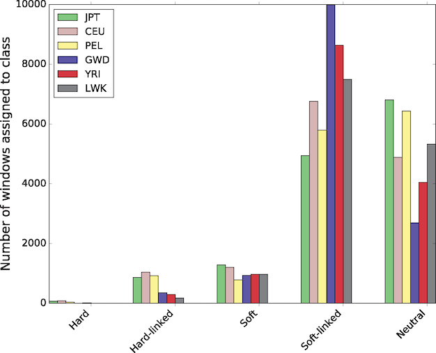
Figure 9: The number of windows assigned to each class by S/HIC in each population.

This is a new technique based on simulated training data. Schrider and Kern acknowledge that their results

may be surprising given the apparently small effective population size and low nucleotide diversity levels in humans. However, if the mutational target for the trait to be selected on is fairly large, then the probability of a population harboring a mutation affecting that trait may be appreciable.

Variance in \(N_e\) can also be important in determining the relative importance of hard vs. soft sweeps (Messer and Petrov 2013). \(N_e\) estimated from sequence data can be dominated by short phases during which \(N_e\) was small, even though \(N_e\) was large for long periods during which adaptation by positive selection was much more likely.

In summary, human adaptation by natural selection was often via soft sweeps, in which \(N_e\) plays a much smaller role.

The effects of population structure on the substitution rate

Another consideration is that the population genetics models of the effects of \(N_e\) and \(s\) on substitution rates make simplifying assumptions, such as random mating (i.e., a lack of population structure), that might easily be violated in real populations. Recent theoretical work has found that population structure can either suppress or amplify the effects of selection (e.g., Frean et al. 2013).

Phenotypic evidence for human evolution

The final piece of background information to keep in mind is the physiological, morphological, and behavioral evidence for human evolution that has informed the studies of evolutionary biologists from Charles Darwin in the 19th century to entire departments of evolutionary biologists in the 21st.

Perhaps the two most dramatic phenotypic examples of human-specific adaptations are (1) bipedalism, and (2) the substantial increase in brain size in humans relative to hominin ancestors and extant apes, most of which occurred since the first appearance of Homo over 2 million years ago (Figure 10):

Figure 10: The evolution of primate cranial capacity. Each dot is a fossil specimen. The x-axis is on a log scale. From Schoenemann (2013)

Two recent studies of variation in cranial dimensions in apes and humans (Weaver and Stringer 2015; Schroeder and von Cramon-Taubadel 2017) found that, whereas great ape cranial evolution was largely characterized by strong stabilizing selection, the divergence of Homo from its last common ancestor with chimpanzees was explained by strong directional selection.

The ability to learn language is a widely accepted cognitive difference between humans and chimpanzees that is probably rooted in human encephalization, as might be the cognitive abilities underlying cumulative culture, which is arguably a uniquely human trait (for a review of the evidence for cumulative culture in humans and other animals, see Dean et al. 2013).

The key point here is that there is overwhelming phenotypic evidence that human psychology did evolve under positive natural selection.

Detailed comparisons of other important aspects of human and great ape phenotypes are available in the Matrix of Comparative Anthropogeny (MOCA) of the Center for Academic Training and Research in Anthropogeny (CARTA).

Empirical evidence that links genetic evolution with phenotype evolution

We are only at the beginning of very long quest to link phenotypes, including the evolved behavioral and cultural phenotypes that are the topic of Casey’s course, to the genome, the focus of the SDSU biologists’ letter. Nevertheless, we know a lot more today than we knew 10 or even 5 years ago.

Functional vs. junk DNA

Genomes can be divided into two parts: functional DNA, which plays a profound role in the phenotype, and “junk” DNA, which plays no role in the phenotype. Functional DNA comprises protein coding regions and non-coding regulatory regions. We now have a pretty good understanding of which DNA sequences code for protein. It is much more difficult, however, to distinguish regulatory DNA from “junk” DNA, and hence to determine the fraction of the genome that is functional, and therefore subject to evolution by natural selectione.

Most attempts to distinguish functional from junk DNA involve identifying sequences that are conserved across species, and are therefore presumed to be under purifying selection (constrained sequences) and thus functional, vs. those that are not conserved across species and so presumably have not been under purifying selection and are therefore likely non-functional “junk” (c.f., ENCODE).

A recent estimate (Rands et al. 2014) is that 8.2% (7.1–9.2%) of the human genome is functional (constrained). Protein coding sequences comprise about 1% of the genome, and are highly conserved across the mammals (Figure 11, red). Non-coding regulatory sequences have much higher rates of turnover (turnover refers to the loss or gain of purifying selection at a particular locus of the genome caused by changes in the physical or genetic environment, or mutations at the locus itself, that switch it from being functional to being non-functional or vice versa). See Figure 11:

Figure 11: Schematic summary of the fraction of constrained sequence that has been retained (saturated colours) or turned over (pastel colours) in the human lineage over time (X-axis, divergence time) and how it has been distributed across various categories of functional element. In addition to showing the reduced quantity of preserved constrained sequence with increasing divergence, we infer the reciprocal quantity of sequence that is assumed to have been gained over human lineage evolution. Figure and caption from Rands et al. 2014.

Because \(>90\%\) of the human genome appears to be non-functional, sequence variation in this portion should closely follow the neutral model. Our focus, then, is on the evolution of the \(\sim 8\%\) of the genome that is functional.

Conserved traits

Perhaps the most important point is that evolutionary anthropologists are keenly interested in the adaptations we share with primates, mammals, vertebrates, and so on. Examples include lacation, the immune system, vision and bitter taste and other plant toxin defense mechanisms that are central to Casey’s research. The major features of these adaptations evolved long before the appearance of Homo, with its small \(N_e\), but would need to have been maintained by purifying selection during the evolution of Homo.

Much of the genetic basis of adaptations we share with other mammals and primates almost certainly lies in the \(\sim 2\%\) of constrained sequence we share with all other mammals and the \(\sim 6-7\%\) we share with other primates (out of 8.2% total; Figure 11).

Moreover, many complex adaptations have evolved features that enable them to adjust ontogenetically to local environmental conditions, an ability that I and many others have framed in strategic terms. Examples include the immune system and induction of xenobiotic metabolizing enzymes. Humans would not be doing too horribly in a wide range of environments even if there were no human-specific adaptations.

Human-specific selection in regulatory sequences

Despite the low \(N_e\) in Homo, there is increasing genetic evidence for positive natural selection in the human lineage since our divergence from chimpanzees. Given that protein-coding sequences are highly conserved across the mammals, and that most functional DNA comprises regulatory sequences, most human-specific adaptations should be grounded in changes to regulatory sequences.

Human accelerated regions (HARs) are short, evolutionarily conserved DNA sequences that have acquired significantly more DNA substitutions than expected in the human lineage since divergence from chimpanzees. HARs are often, but not always, the product of positive natural selection (other mechanisms include relaxation of constraint, which allows a region to acquire more mutations than it would under purifying selection, and GC-biased gene conversion; Franchini and Pollard 2017).

Franchini and Pollard 2017 summarized multiple studies that attempted to discover HARs, which differed in the number of species considered to determine “conserved” (which ranged from a few primate species to multiple primate, mammalian and vertebrate species), sequence filtering criteria (e.g., including or excluding coding sequences), and statistical tests for acceleration. Although each study identified a large number of HARs, there was only limited overlap in the identified regions. See Figure 12:

Figure 12: Identification of human accelerated elements. Top: the four different approaches used to identify human accelerated regions. Some key differences include (i) the conserved elements used as candidates to identify HARs (which depend on multiple sequence alignments, methods to detect conservation, and whether human was masked in the alignments), (ii) bioinformatics filters that aim to restrict to non-coding elements and/or remove assembly or alignment artifacts, and (iii) tests used to detect acceleration. Bottom: overlap of the different datasets of human accelerated regions. Abbreviations: ANC accelerated conserved non-coding sequences [20]; HACNS human accelerated conserved non-coding sequences [23]; HTBE human terminal branch elements [21]. HARs include the original HARs [19] and the second generation HARs or 2xHARs [100]. Figure and caption from Franchini and Pollard 2017.

Most studies of HARs used only sequence data. Some recent studies, though, also incorporated expression data. Gittelman et al. 2015, for example, used maps of DNase I hypersensitive sites (DHSs) from ENCODE and the Roadmap Epigenomics Projects. DHSs are regions of chromatin that serve as markers of regulatory DNA. Of 2,093,197 DHS loci, 113,577 exhibited significant constraint across the primates. DHSs active in fetal cell types, especially fetal brain cells, showed the highest levels of conservation in non-human primates. Of the conserved loci, 524 were accelerated in human evolution (haDHSs), evolving at approximately four times the neutral rate in the human lineage, mostly but not exclusively under positive selection, while other primate lineages evolved at less than half of the neutral rate. Gittelman et al. found that haDHSs tend to target developmentally and neuronally important genes relative to conserved DHSs, which themselves are already highly enriched for these categories.

In another review of several previous studies of HARs, Levchenko et al. 2018 noted that of the 3500 candidates identified so far, most are in non-coding regions, estimates of the fraction under positive selection range from 15%-85%, many are active in the brain, consistent with this major phenotypic difference between humans and chimpanzees, and about 7-8% are not shared with Neanderthals or Denisovans, consistent with the time of their divergence from the modern human lineage.

Recent human evolution

Human \(N_e\) started a dramatic increase some 40-50,000 years ago as humans entered multiple new environments. Hawks et al. (2007) predicted and found that “selection has accelerated greatly during the last 40,000 years.” Co-authors Cochran and Harpending followed up with a book, The 10,000 year explosion: How civilization accelerated human evolution (you can find my review of it here). Fan et al. (2016) review many examples of recent, population-specific human adaptations to local environments, such as the arctic, tropical rainforests, and high altitude:

Figure 13: Examples of human local adaptations, each labeled by the phenotype and/or selection pressure, and the genetic loci under selection. Figure and caption from Fan et al. (2016).

Wrap up

Evolutionary anthropologists and human behavioral ecologists investigate the relationships between human environments and humans’ intricate molecular, cellular, anatomical, and behavioral phenotypes, most of which we inherited from primate, mammalian and earlier ancestors that evolved long before our lineage experienced a low \(N_e\). The extent to which a small \(N_e\) limited human-specific evolution is still under investigation. It certainly didn’t reduce it to zero, and there are many other factors that might have accelerated it. There is abundant phenotypic evidence for human-specific adaptations, after all, and there is increasing genetic evidence that positive selection played an important role in our evolutionary history, especially selection on standing variation, which is not limited by low \(N_e\).

Reading through the papers I discussed here, I was encouraged that folks studying human genetic variation seemed interested in, not hostile to, the many adaptationist hypotheses put forward by evolutionary anthropologists and behavioral ecologists. Charlesworth and Charlesworth, for instance, highlight the importance of kin selection and evolutionary game theory, two theoretical foundations of behavioral ecology. O’Bleness et al. (2012) give a nod to Lieberman’s endurance running hypothesizes and many other phenotypic comparisons of humans and non-human primates.

So what’s up with the SDSU biologists? The debates over adaptationism and neutralism vs. selectionism have all the hallmarks of a sectarian conflict. Contrary to our rhetoric, academics are among the most ethnocentric of an infamously ethnocentric species. Perhaps — dare I say it? — ethnocentrism is part of human nature. If so, it’s true of us all.

But, among the primates, our species also evolved a unique ability for group alliances. The SDSU biologists are doing cool stuff. Casey is doing cool stuff. Knowing Casey as I do, he doesn’t need my advice, but I’ll give it anyway: I doubt the SDSU biologists speak with one voice. There is as much diversity of opinion within groups as there is between them, maybe more. You are one of the very few SDSU social scientists who has a professional interest in what the SDSU biologists are doing. I suspect many of them recognize that.

2018/7/15: minor edits to this post to improve clarity.

---

1. There is debate about the human mutation rate. See Scally and Durbin 2012 and Scally 2016.↩︎